When you don’t know your edge, how much should you stake?

In May 2020, two shareholders (Andrés Barge-Gil and Alfredo García-Hiernaux) of the tipster platform Pyckio published a paper in the Journal of Sports Economics addressing how a profitable bettor should stake under conditions where estimates of the true probabilities of winning are unavailable.

Whether a bettor aspiring to be consistently profitable over the long term should even be active under such conditions is a moot point, although Barge-Gil and García-Hiernaux have suggested that many sports bettors acknowledge that they are unable to estimate them accurately.

Nevertheless, their research is interesting in as much as it casts a light on how different staking plans can be reinterpreted as variants of the Kelly criterion. In this article, I want to summarise their efforts and look at whether what they found can actually be improved upon.

Reinterpreting different staking plans with Kelly

There is perhaps no more popular topic in the world of sports betting money management than using the Kelly Criterion as a staking method. Indeed, Pinnacle’s Betting Resources has numerous articles on the subject. I myself have written a couple. In particular I demonstrated that for simple Kelly staking where only one bet at a time is placed before settlement, the strategy is able to accommodate the risks of not knowing precisely your advantage on a bet-by-bet basis so long as you are accurate on average.

In their paper Barge-Gil and García-Hiernaux have suggested that when precise estimations of true bet probabilities are unknown, bettors abandon Kelly and resort to different money management plans.

Unit loss

The first of these is the unit loss, or level stakes, method, where the bettor risks the same stake on every bet regardless of the odds. The longer odds, the bigger the impact on the bankroll in the event the bet wins, but the lower the likelihood that the bet will win.

We can reframe unit loss staking as a Kelly plan where the expected value or yield is linearly proportional to the odds. Since the size of the Kelly stake is given by EV / odds – 1 (where EV is the expected value, with anything over 0 considered profitable), a unit loss plan implies that this ratio remains constant.

For example, suppose EV was 10% (0.1) and the odds 2.00. The stake would be 0.1. If the odds increase to 4.00, this implies that the EV must increase to 30% (0.3) to ensure that the stake remains at 0.1. Odds of 101.00 would imply an EV of 10 or 1,000% which seems a tad unrealistic. That would imply true odds of only 9.18. Surely no bookmaker’s going to make such a big mistake.

Indeed, in the limit that the odds tend towards infinity, the true odds would tend towards a maximum value given by 1 / stake, in this case 10. A major critique of unit loss staking is that it places too much risk on longshots with low win probabilities. For Kelly advocates, it would only make sense if EV really did increase proportionally with odds, and as we can see this is hardly credible.

Unit win

The second money management plan typically used by bettors is unit win staking. Here, the stake is such that the bettor aims to win the same profit regardless of the odds. If the target win, or profit, was €100, odds of 2.00 would require a €100 stake, whilst odds of 5.00 would require a €25 stake. The stake size is proportional to the reciprocal of the odds – 1. In terms of Kelly, the unit win strategy implies that EV is completely uncorrelated with the Kelly Criterion; all EVs are the same regardless of the betting odds.

As for unit loss staking, something doesn’t seem quite right. Could it really be the case that a bettor’s advantage will be the same, whether the odds are 1.11 or 111.00? The lessons from variance would suggest this doesn’t seem very realistic. Indeed, if your EV at odds of 111.00 was 20% (0.2), the same EV at odds of 1.11 would imply the true odds were less than 1, plainly complete nonsense. Something can’t have an outcome probability of greater than 100%.

Unit impact

Barge-Gil and García-Hiernaux have proposed an alternative staking plan: unit impact, under the hypothesis that this plan fits better with the Kelly staking method. The unit impact method holds constant the difference in the bankroll between winning and losing and is the same no matter how long or short the odds.

The unit impact stake is proportional to the reciprocal of the odds, in contrast to unit win which is the reciprocal of the odds – 1. Thus, if the stake is €100 for odds of 2.00, the unit impact stake for odds of 5.00 would be €40. For each case, the difference between winning and losing is €200 (+€100/-€100 in the first case and +€160/-€40 in the second case).

For unit impact staking, EV is proportional to odds – 1 / odds. This means that EV increases with increasing odds but at a decreasing rate towards a limit, since this ratio quickly tends towards 1. For example, if EV = 0.1 for odds of 2.00, the limit in EV will be 0.2. Whilst this scenario is not as extreme as for unit win staking where EV remains unchanged, it again seems to underestimate the possibility of higher EVs for longer odds.

Successful racing tipsters are typically seen to have yields considerably more than double those focused on the Asian Handicap market or point spreads, although this does not necessarily imply there are any more skilled (or luckier); they just have greater variance on their side.

Following Barge-Gil and García-Hiernaux the chart below illustrates how EV varies with odds for the three different staking plans, assuming that EV = 3% for odds = 2.00 for each.

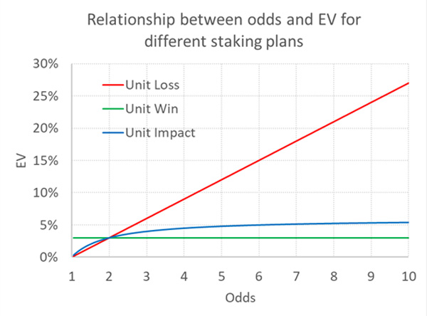
As previously argued, the unit loss and the unit win staking plans both seem to imply unrealistic relationships between odds and EV.

Barge-Gil and García-Hiernaux have analysed Pyckio’s betting picks database and believe they have confirmed that the EV–odds relationship implied by unit impact staking best reflects both observed and expected tipster yields (the latter based on closing prices). I remain somewhat unconvinced. To reiterate, unit impact staking will still only ever produce an EV that is at most double the EV for odds = 2.00. Is there a better alternative?

Revisiting the t-distribution

Three years ago, I introduced to Pinnacle’s Betting Resources the use of the t-distribution when evaluating betting tipsters and deciphering luck from skill. Similar to the normal distribution (and used instead of it when only the sample rather than the population standard deviation is known) it can help determine how unlikely a given sample is assuming the population mean is known.

I have used the t-distribution extensively in my work to help bettors show how likely their betting records could have happened by chance, assuming they had no skill. The smaller the probability, the more subjectively confident you can be that it wasn’t only chance that had anything to do with your betting profits.

At the heart of this test is the t-statistic or t-score, from which the probabilities can be derived. I have shown that for unit loss staking, and where the betting odds of your record don’t vary too much, this statistic can be approximated with the following formula.

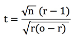
where n is the number of bets, o the average odds and r the return on investment or yield + 1.

Like the z-score, which handicappers may be more familiar with, it is essentially a measure of the number of standard deviations your betting yield departs from an expected mean of zero, if betting unskilled and to fair odds. A t-score of 2, for example, would imply that a better yield than the one achieved by your record would only be expected about 2.5% of the time, assuming you had no skill. The t-score is thus a type of likelihood measure. The bigger the t-score, the less likely the observation. Let’s use it to see how likely different EVs are (assuming no skill) depending on the odds we are betting.

The asymmetry of returns

Suppose you bet a team with an 80% chance of winning, with fair odds 1.25. Suppose now the bookmaker wrongly believes the win probability is 75%. He’s running a promotion and has no margin. His odds are 1.333. Accordingly, your EV is 6.667% (1.333/1.25 – 1 or 0.80/0.75 – 1).

Now consider a second scenario: the true chance is 20% (fair odds of 5.00) but the bookmaker believes it to be 15%, (published odds of 6.667). This time your EV is 33.33% (6.667/5.00 – 1 or 0.20/0.15 – 1). The difference in expected win percentage between your estimate and the bookmaker’s is the same, but the EV is 5 times as large. It seems in terms of EV, equivalent errors are punished more heavily the longer the odds are. But how likely are those errors?

The symmetry of likelihood

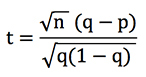
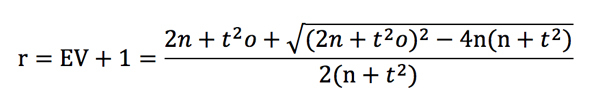
Let’s rewrite the t-score formula above (assuming all our bets have the same odds, o). Since we know that r = q / p, where p is the implied probability of the bookmaker’s odds (i.e. 1/o) and q is your estimated probability (which is ‘true’ if your forecast model is accurate), then it can be shown that:

Suppose n, our number of bets, is 100. For q = 0.8 and p = 0.75, t = 1.25. Similarly, however, for q = 0.2 and p = 0.15, t = 1.25 also. Assuming the bookmaker, and not our model, was actually correct, such a t-score would correspond to an outcome probability of 10.7% (using Excel’s =TDIST function).

Over 100 bets we would expect to do better than 6.667% yield at odds of 1.333, or better than 33.33% at odds of 6.667, 10.7% of the time. Bigger yields at longer odds are just as likely as smaller yields at shorter odds; hence why racing tipsters have the illusion of looking better than handicappers, or much worse if they are losing ones.

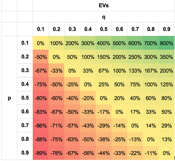
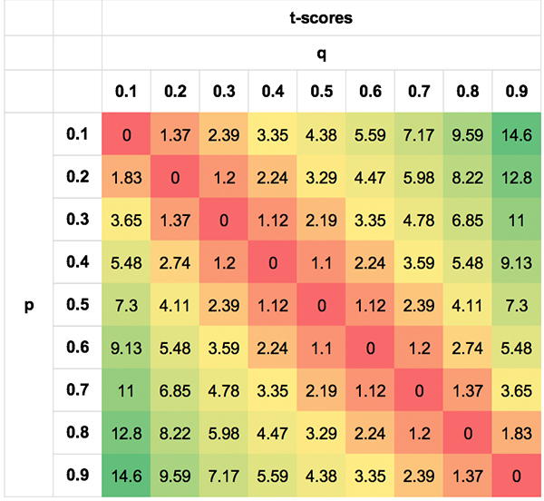
I’ve attempted to show this likelihood symmetry by means of the following tables. The values are extreme simply to illustrate the point; obviously; no bettor will be able to do this well, or badly, for most of the scenarios.

The first shows the asymmetry in EV for different p, q pairs. The second shows the symmetry in the t-scores. I’ve shown the absolute t-scores (removing the negative sign for negative EVs when q < p) for visual clarity. Not only is a p, q pair of 0.3/0.7 equally likely as a pair of 0.7/0.3, but so, too, are pairs like 0.7/0.5 and 0.3/0.1, 0.8/0.7 and 0.2/0.1 for the reasons described above.

A new EV–odds function

For given odds and EV there is a likelihood t (which doubles as the number of bets increases 4-fold). We can rearrange the t-score formula to express it in terms of r. This leads to a rather horrible quadratic with an even more horrible solution.

That’s a whole lot nastier than odds – 1 / odds but let’s plot it nonetheless for the scenario where EV = 0.03 and odds = 2.00. This is shown below, along with the previous EV–odds functions for unit loss, unit win and unit impact staking.

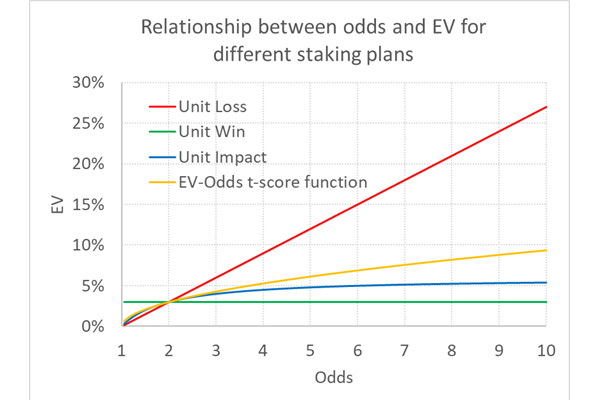
Whilst the function might be difficult to write, it makes more intuitive sense given that it interprets expected yields in terms of statistical likelihood. For unit impact staking, EV can never be greater than 6% when it’s 3% for odds of 2.00. But with my function it can grow indefinitely, albeit not as unrealistically fast as for unit loss staking, but in line with that predicted by statistical variance. For odds of 10 it is 9.4%, for odds of 50 it is 23.3% and for odds of 1,000 it is 150%.

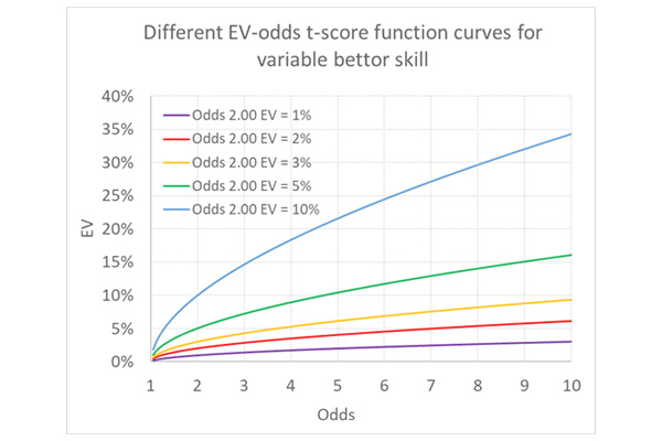
One obvious criticism is that this function, based as it is on the t-score, assumes the bettor has no skill. It is simply expressing the likelihood of things happening assuming no skill is present. But this is a misreading; even if skill is present, the same statistical laws associated with variance apply.

The position of the orange curve would change, but the shape would remain the same. I’ve shown some possible trajectories below for bettors with varying degrees of good luck or skill, whichever you want to call it. The original curve for the bettor with EV of 3% at odds of 2.00 is still shown in orange.

An additional criticism might be that we are also assuming any skill would independent of the odds, that is to say the same whatever they were. Given market inefficiencies like the favourite–longshot bias, that may not be an appropriate assumption.

Testing the function

Can we test the validity of this new EV–odds function? My Wisdom of the Crowd betting system, which those who follow me regularly via Twitter and Football-Data will know all about, uses Pinnacle’s more efficient odds to estimate the EV available in odds from other bookmakers.

Using a sample of match odds data from European domestic league football dating back to the 2012/13 season, I found 55,237 occasions where a profitable EV (>0) was available. The average was 2.20% (for the record the actual performance from unit loss stakes was 1.77%, well within the statistical margins of model error), with average odds of 3.30. With these figures we can use my quadratic solution formula to construct an EV–odds function curve like those above. This is the orange one below.

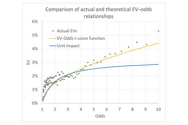
Compare this firstly to the actual model EVs averaged by 1%-win expectancies (shown as odds in the chart), and secondly to the EV–odds function curve predicted by unit impact staking. Whilst not a perfect match, the EV–odds t-score function arguably does a much better job at predicting ballpark EVs based on betting odds.

A rationale

The observant amongst you might now say: what on earth is the point of using an EV–odds function to predict the EV for different odds when your Wisdom of the Crowd model does that explicitly for every bet? This is indeed a valid judgement, and much of this article could thus be considered rather theoretical.

Nevertheless, even accurate models (on average) exhibit epistemic uncertainty on a bet-by bet basis. Furthermore, aleatory (or inherent) uncertainty renders the assessment of true win probabilities practically impossible.

The purpose of this exercise, then, as it was for Barge-Gil and García-Hiernaux, was to illustrate how one might attempt to ballpark estimate your EV where you recognise those quantitative uncertainties, when your prediction model doesn’t explicitly estimate win probabilities, or where your method of forecasting is more qualitative via hunches rather than data crunching. Know your odds and with this method you can estimate your EV; know your EV and you can then determine what Kelly stake you should use.

This t-score methodology might well be convoluted but its outputs are derived from a more intuitive reasoning of the relationship between win probability, expected value and outcome likelihood, and by extension, how actual yields may be seen to vary with betting odds. For advocates of Kelly, I think it works better than unit impact staking, and certainly better than unit loss and unit win.

MORE: TOP 100 Online Bookmakers >>>

MORE: TOP 20 Cryptocurrency Sportsbooks >>>

MORE: Best E-Sports Betting Sites >>>

Source: pinnacle.com