The Monte Carlo method relies on repeated random sampling to obtain numerical outputs when other mathematical approaches would prove to be too complicated. They are particularly useful for bettors less familiar with traditional statistical testing methods as they require little mathematical knowledge.

Dominic Cortis has already discussed how it might be applied to sports prediction, considering a specific example of forecasting the Formula 1 championship. Here, I’m going to use it to investigate how I might expect my betting performance to vary as a consequence of chance.

Analysing your betting performance

A betting history from my Wisdom of Crowds methodology that I will use in this article contains 1,521 bets and shows a profit over turnover to level stakes of 0.76%. But how do I know whether this represents a par, lucky or unlucky performance?

The first step is to compare this to expectation. Implicit in the methodology is the estimation, for each bet, of the fair betting odds and consequently the amount of value expectation held. For example, for fairly priced odds of 2.00, a published betting price of 2.10 would offer me a value expectation of 5% or 1.05 (calculated by 2.10/2.00).

A fair price of 2.00 implies a win probability of 50%. If I win 50 out of 100 such bets, making a profit of €1.10 for each, whilst losing 50 bets for a loss of -€1 each, my net profit is $5 (or 5% of a €100 turnover). Similarly, published odds of 3.50 for a fair price of 3.00 would hold a value expectation of 16.67%. The table below shows the selections my betting system identified.

*Pinnacle odds with the margin removed

For a complete betting history it is easy enough to determine the overall value expectation and the expected profit as you simply calculate the average. For my history of 1,521 bets, this was 4.04%, implying that if my betting system was behaving exactly as I had predicted, my expected profit would have been €61.45 from €1,521 wagered.

In reality, the history was showing a return of €11.61. Evidently, it had underperformed on account of bad luck - assuming, of course, my forecasting model was working as it should. The question is by how much. This is where Monte Carlo can help.

Running a Monte Carlo simulation in Excel

Running a Monte Carlo simulation in a software package like Excel is relatively straightforward:

1. Calculate the expected probability of a win for each bet, expressed as a decimal between 0 and 1. This is simply the inverse of the fair odds.
2. Use Excel’s RAND function to output a random number between 0 and 1 for each bet. To determine whether each bet wins or loses in our simulation, we simply ask Excel whether the random number associated with each bet is less than the expected win probability. If it is, we assign a level stakes profit equal to the odds – 1. If it’s not, we assign a level stakes loss of -1.
3. Sum the individual profits and losses for all bets in the simulation to calculate the yield. For level staking, simply divide the profit total by the number of bets
4. Use Excel’s Data Table function to refresh the random numbers for a specified number of simulations.

The first two steps for my bets are shown below.

Pressing the F9 key will recalculate all the random numbers for a completely new simulation and a new theoretical sample yield. We could manually make a note of the yield each time we run a new simulation, but if we want to do this hundreds or thousands of times, this will prove to be laborious and time consuming.

Thankfully, Excel offers us a quick and easy method to run many simulations in one go, by using its Data Table function. You will find this in Data > What If Analysis > Data Table:

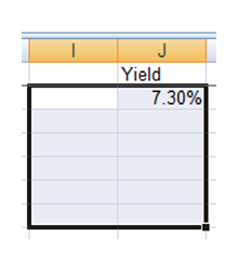
1. 1. Calculate your yield for your sample in any free Excel cell as described in step three above.
   2. Next, highlight a number of cells which you wish to populate with yield values for new simulations along with a single column to the left.

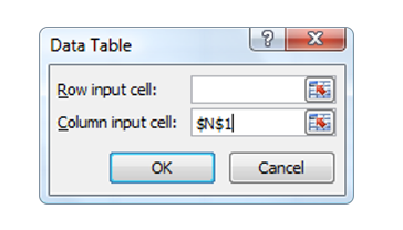
1. 1. Next call up the Data Table in Excel. You will see a box like the one below. In the Column input cell, simply type a single cell reference. It can be any cell, provided it’s not one of your highlighted cells from the previous step.
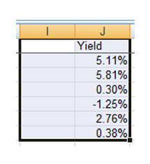
   2. Click OK and watch Excel run its magic. The highlighted cells beneath your first one will be populated with new calculated yields, each one representing a single simulation run. In this example, I’ve produced six simulations, as shown below.

Measuring the effect of luck on your betting profits

Dr. Gerard Verschuuren has produced a very helpful YouTube tutorialdescribing this process in more detail. We can run as many simulations as we wish, although the larger the number the longer Excel will take to perform the calculations. For the purposes of this article, I have run 100,000 simulations (which took about five minutes).

Another key point to take away from this exercise is the influence bad luck can have on positive expectancy bettors over fairly sizeable betting histories.

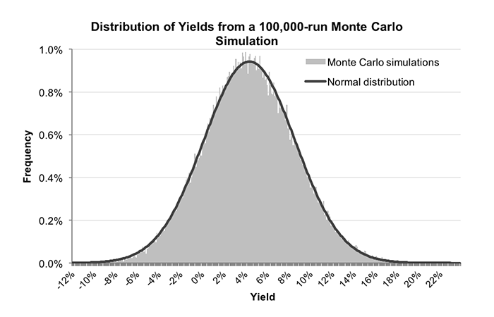
The average yield was 4.05%, almost exactly the same as the value expectation for my betting history. However, there was a wide variation, from the worst performance of -12.23% to the best performance of 23.26%.

Indeed, almost 17% of simulations actually returned a loss despite my betting history holding a theoretical value expectation of over 4%, whilst my actual yield of 0.76% could be expected to be surpassed on 78% of occasions.

In fact, with this data we could use Excel to calculate the probability of achieving any particular yield threshold, without the need to resort to any statistical testing. The Monte Carlo method has done all that for us. The full distribution of 100,000 simulated yields is plotted in the chart below (with 0.1% increments along the x-axis). For those familiar with the normal distribution, you can see that it is an almost perfect match.

Of course, if my actual yield had been, say, -5% or worse (which would be expected to happen on just 1% of occasions), I might start to wonder whether my betting system was actually flawed instead. The Monte Carlo method, then, is clearly a useful tool to help with such subjective evaluations.

A flawed betting system vs. Bad luck

Another key point to take away from this exercise is the influence bad luck can have on positive expectancy bettors over fairly sizeable betting histories. My history was over 1,500 bets in size and held a predicted expectation of over 4%. Despite this advantage, my Monte Carlo simulations demonstrated that I could still end up losing in over one in five occasions.

If you held a similar advantage with your betting strategy how would you be feeling after 1,500 bets and nothing to show for them: confident in your methodology, putting the underperformance down to bad luck, or losing faith in your whole approach?

One way to help resolve such a dilemma is to increase the sample size. Again, we can play with the Monte Carlo method to see how things change when a betting history grows, As a thought experiment I increased my original 1,521 bets tenfold (simply by repeating the original sample of betting odds nine additional times). Performing another 100,000-run simulation yielded the following figures:

• Average yield = 4.04%
• Lowest yield = -1.21%
• Highest yield = 10.17%
• Probability yield < 0% = 0.1%
• Probability yield > 0.76% = 99.3%

The new distribution of 100,000 simulations is shown below, superimposed over the original distribution for the original sample of 1,521 bets.

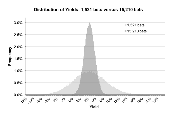
The obvious difference between the two samples is the size of the spread or range of possible yields, being much narrower for the larger betting history. Such an outcome is entirely predictable and is simply a consequence of the law of large numbers.

Assessing the Monte Carlo simulation results

The larger my betting history, the more probable it is that the actual performance will be closer to expectation, assuming, of course, that my prediction methodology is working as it should. The corollary is that, should I still be showing a yield of 0.76% or worse after over 15,000 bets, I would seriously begin to question whether it was.

Ultimately, the Monte Carlo method will not be able to tell you definitively whether your betting system possesses anything beyond the influence of chance. Nevertheless, it does provide a useful tool to help guide you towards an informed judgement in that respect, whilst illustrating the range of possible outcomes you might reasonably be expected to witness within the confines of good and bad luck.

MORE: TOP 100 Online Bookmakers >>>

MORE: TOP 20 Bookmakers that accept U.S. players >>>

MORE: TOP 20 Bookmakers that accept Cryptocurrency >>>

Source: pinnacle.com