What is a betting system?

In contrast to a staking method or money management strategy, which proposes a method of assigning stake sizes to your bets, a sports betting system is a structured prediction methodology built on a quantitative analysis of historical data designed to overcome the bookmaker’s profit margin and find positive expected value.

Bettors frequently confuse money management and betting systems – search for ‘betting system’ on Google and most of what you’ll find are strategies like Martingale, Labouchere or Fibonacci – but really they are different things.

Money management simply changes the nature of risks associated with your bets; it cannot, however, turn a losing prediction method into a winning one over the long term. A betting system, by contrast, attempts to find the ‘true’ probabilities of things happening in a sporting contest.

Sports betting systems: Regression analysis

The most widely used method for designing a sports betting system is statistical regression analysis. To those not familiar with statistical jargon this can sound intimidating but really it’s just a method of estimating the relationship between variables.

Whilst regression analysis is a useful tool for designing a betting system, its underlying weakness is its inability to distinguish between correlation and causation.

The simplest of these is simple linear regression where just two variables are considered, for example the number of goals a team scores (the predictor or independent variable) and their match win frequency (the response or dependent variable).

In my first book Fixed Odds Sports Betting: Statistical Forecasting & Risk Management I discussed a simple regression model based on the relative goal supremacy of two teams over their previous 6 games.

Using a large sample of matches (in this case 8 seasons from 1993 to 2001) it is possible to plot a chart correlating the calculated match ratings (the home side’s 6-game goal difference minus the away side’s 6-game goal difference) with the frequency of each match result. The distribution of match rating (the independent variable) versus home win frequency (the dependent variable) is shown below.

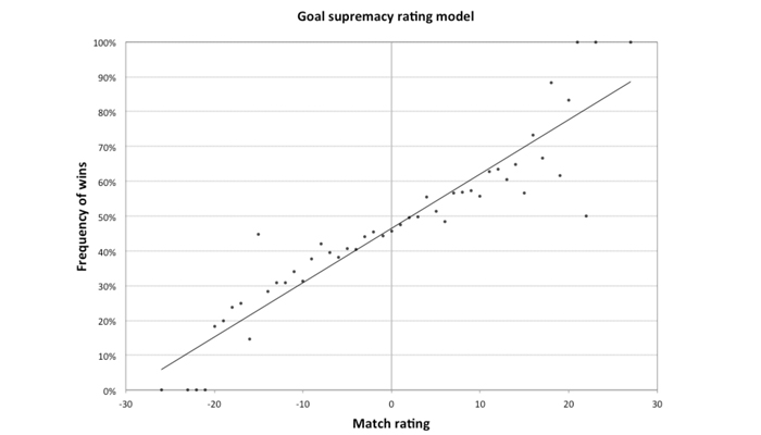
Whilst the individual data points in the chart are somewhat scattered, there is an obvious linear trend relating the two variables: the better the home team relative to the away team in terms of their last 6 games’ goal difference, the more likely it is that the home team will win the match.

The regression line drawn on the chart essentially describes an idealised relationship between relative goal supremacy and the home win frequency with the noise or random good and bad luck removed.

We can describe the aforementioned line by means of an equation; being a simple linear regression model, it takes the form y = mx +c, where y is the dependent variable (the win probability), x is the independent variable, the match rating, m, is the slope or gradient of the trend line (and a measure of the strength of the relationship) and c is the constant or point at which the line intercepts the y-axis (i.e. x = 0). In this example, the equation is given by:

When the match rating is zero (that is to say the home and away teams are more or less evenly matched in terms of goal difference) the win probability is 46.5%. This seems intuitively sensible, given that about 46% of football games finish with a home win. Where the home team has a net goal difference of ten more than the away team over the past six games, the regression model shows that such teams typically win 62% of the time. With a 20-point superiority, this rises to 78%.

Our regression analysis can also tell us how much of the variability in the win frequencies is explained by this betting system model. In this case it was 86%. You can see this illustrated by the goodness of fit of the trend line to the data. It tells us that there is a strong correlation between the two variables.

Using a system to making betting predictions

To turn our regression model into a fully functioning betting system, we now need to make predictions about future matches and use them to identify bets that hold positive expected value.

As with most modelling methodology, the standard assumption is that the past is the key to the future. If previous matches with match ratings of +10 ended with a home win 62% of the time, then the assumption will be that a home team with a 10-point goal supremacy over their opposition will have a 62% probability of winning the match.

We can then simply translate these probabilities into the ‘true’ odds, and hence find expected value at a bookmaker that offers longer odds. Applying this model to the 2001/02 English football league season I managed to achieve a profit over turnover of +2.1% from 526 wagers at best available home win betting odds, compared to a loss of -3.7% if I had simply bet all home wins in that season blindly.

Correlation vs. Causation

One season’s betting with a little over 500 wagers doesn’t guarantee profitability can be reproduced season after season. It may seem like an adequate number to be sure of a reliable betting system but regular Betting Resources reader will know this isn’t the case.

Pinnacle’s article on the law of small numbers serves as a reminder that even samples of 1,000 wagers can reveal illusory patterns of profitability which in fact have no basis in causality, but merely arise by chance. Sadly, the following five seasons using this betting system all returned losses.

Whilst this simple goal supremacy regression model did a great job of finding which home teams were more likely to win, it didn’t guarantee that it could find teams that were more likely to win than the probabilities implied by the bookmakers’ odds.

Unfortunately, many sports bettors often misinterpret precision, accuracy and validity when studying their betting history, confusing correlation and causation in the process.

My model might have been good at forecasting, but seemingly it wasn’t better at forecasting than the models used by the bookmakers to set their odds, nor indeed better than the models used by other bettors that helped shape and shift those odds.

If my model was simply replicating what the bookmakers’ models were doing, profitability will show no persistence and simply reflect the vagaries of randomness. It appears it was not built on any valid correlation. My model predictions did not ‘cause’ those profits because it was not more accurate than other models doing the same thing.

Precision vs. Accuracy

Of course, a two-variable linear regression model is hardly the most sophisticated of betting systems to try to find expected value. Multiple regression, where more independent or predictor variables are introduced, offers a means of increasing forecasting precision. However, analysts should be wary that this is not at the expense of accuracy.

A precise model is one where measurements are close to each other, for example as illustrated by the trend line in my simple linear regression model above. Precision, however, does not guarantee accuracy. Accuracy is a measure of how close you are to the ‘true’ value. Precision is associated with random errors and accuracy with systematic ones (otherwise known as bias).

For a betting system to be valid, that is to say to be really doing what it is supposed to be doing (i.e. consistently finding profitable expected value) it must be both precise and accurate. Validity implies both predictability and persistence, that is to say whether what we think is the cause is actually the true cause and whether our measurement repeatedly points to that conclusion.

Unfortunately, many sports bettors often misinterpret precision, accuracy and validity when studying their betting history, confusing correlation and causation in the process. Their error is in believing that profits they have made were ‘caused’ by their betting system when frequently it is the case that they simply arose because of good fortune.

The pitfalls of regression analysis

Whilst regression analysis is a useful tool for designing a betting system, its underlying weakness is its inability to distinguish between correlation and causation. Regression analysis is effective at identifying an association between variables, for example goals scored and conceded versus the probability of winning matches, but it is unable to determine if one causes the other.

Regression analysis might show us that when Barcelona loses, Lionel Messi does not score a goal. However, we cannot conclude that Lionel Messi not scoring is the cause of Barcelona losing the match.

Without establishing causation and validity in our betting system, we should be wary that it may be no better than prediction models used by everyone else. In a relative skills context like sports betting, we don’t get paid for merely predicting the future, we have to be better at that than everyone else.

MORE: TOP 100 Online Bookmakers >>>

MORE: TOP 20 Bookmakers that accept U.S. players >>>

MORE: TOP 20 Bookmakers that accept Cryptocurrency >>>

Source: pinnacle.com