By understanding what to expect over a series of bets, sound bankroll management will assist a bettor in avoiding certain behavioural biases such as Overconfidence Bias, Self-attribution Bias, and The Illusion of Skill, that may erode expected profitability over the long-term. This article explores how odds, edge and variance interact and can help guide bankroll expectations for bettors.

Bankroll management

Managing a bankroll and understanding variance are crucial skills for any bettor. From poker players to sports bettors, traits that all successful bettors will possess include their ability to understand and quantify their edge, and to attribute variance to either good or bad luck.

Consider a bet at odds of 2.0, which implies a probability (no margin) of 50%. If a bettor can accurately determine that the true probability is 52% (true price of 1.92), the expected return for each bet made at 2.0 will be 4% (2.0/1.92 – 1). This can be referred to as the bettor’s ‘edge’.

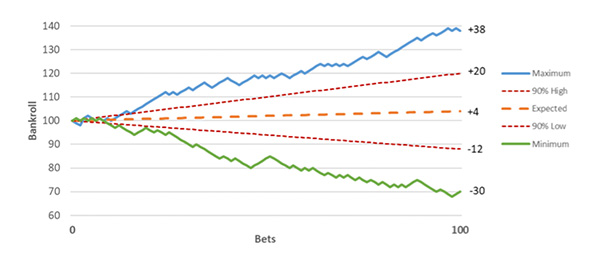
Now let’s assume a bettor starts with a bankroll of 100 units and bets a fixed one unit. After 100 such bets, the bettor’s bankroll could be anywhere from 0 to 200 units, however it is expected to be 104 units - a profit of 4%.

By simulating this scenario 10,000 times we can see the effect of variance on the bettor’s bankroll in the chart below.

Understanding variance

While the average result was just under a four unit increase in bankroll, the difference between the best (+38 units) and worst (-30 units) outcomes is substantial. As a bettor it is important to understand variance and be aware that a 4% edge doesn’t guarantee a 4% profit.

With this simulation of 100 bets, 90% of the time a bettor can expect a return of between -12 units and +20 units. A 10 unit drawdown (from your starting bankroll) can be expected around 20% of the time, however just 2% of the time a bettor will experience a 20 unit drawdown.

Interestingly, 32% of the time a bettor can expect to be down after 100 bets, despite a 4% edge on every bet.

If we increase the bettor’s edge to 10% (true probability of 55% for a wager at 2.0), a loss occurred 13% of the time after 100 bets.

The chance of a drawdown of 20 units or more was just 0.4%. Of course, as the edge increases, the likelihood of a bad run decreases, but what happens when the number of wagers is increased to say 5,000. The chart below shows the first scenario above (52% true probability, betting at odds of 2.0) simulated 10,000 times.

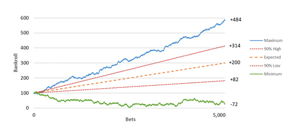
Whilst the worst outcome was bad at -72 units, only 28 (0.28%) of the 10,000 simulations delivered a loss after 5,000 bets. In 90% of simulations a return of between +82 units and +314 units was generated. This reflects a return on investment (ROI) of between 1.64% and 6.28%.

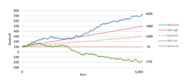
How does the scenario change if instead of betting at 2.0, the odds are 4.0 (implied probability of 25%)? If we determine the true probability to be 26% (true price of 3.846), the expected return for each bet remains the same at +4% (4.0/3.846-1), but what happens to variance?

How do the charts compare?

Comparing the two charts, we can see that variance has increased significantly despite an identical bet size, number of bets and expected return. The standard deviation of returns increased from 1.4% to 2.4%. The range of simulated outcomes is 64% greater in the scenario betting at 4.0, and the 90% confidence range is 72% wider, representing an ROI between 0% and 8%.

In the first scenario, the bettor lost the entire 100 unit bankroll on just 2 of the 10,000 simulations (0.02%). In the latter, the entire 100 unit bankroll was lost in 6.3% of the simulations. A 50 unit drawdown was significantly more likely (25.7%) when backing the 4.0 outsider compared to betting at 2.0 (2.0%).

In the worst scenario betting at 4.0, almost three entire bankrolls (-276 units) would have been lost. What this example shows is that with a constant bet size, number of bets and expected return, variance increases as the odds increase.

As such, a bettor that predominantly backs underdogs can expect to have more and larger swings in their bankroll than a bettor that backs favourites, even if their edge is the same.

Given it may take months or even years for a sports bettor to make 5,000 wagers, it is probably more relevant to understand the bankroll implications whilst making a significantly smaller number of wagers.

Assuming a bettor can find 4% edge at odds of 2.0, and bets a fixed 1 unit, the chart below shows the chance of having a certain unit drawdown from your starting bankroll over a series of between 100 to 1,000 bets, based on 10,000 simulations.

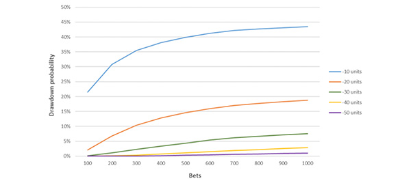
By making 1,000 bets at odds of 2.0 and with an edge of 4%, the chance of experiencing a certain drawdown appears to be approaching its upper limit, especially for smaller drawdowns. As the bettor’s edge increases, the chance of a certain drawdown decreases. The chart below plots this probability for a series of 1,000 wagers at odds of 2.0, based on 10,000 simulations.

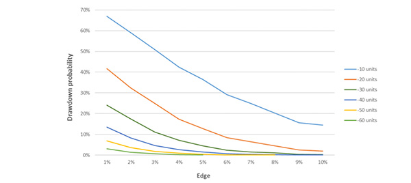
For example, with a 4% edge, the chance of experiencing a 20 unit drawdown during the course of having 1,000 bets at 2.0 was 17.4%. However, the chance of being down 20 units or more after 1,000 such bets was just 2.8%. Understanding this difference will ensure a bettor is able to look through short term variance with a view to their long-term edge.

Different bankroll implications

What are the bankroll implications if we keep the bet size and edge constant but vary the odds? The chart below plots the probability of various drawdowns (from starting bankroll) when a bettor places 1,000 1 unit bets at various odds, with an edge of 4%. Each series of 1,000 wagers was simulated 10,000 times.

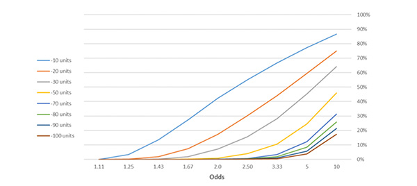
Recall that when betting at odds of 2.0, there was a 17.4% chance of being down 20 units at some stage through a series of 1,000 bets. At odds of 5.0, the chance of a 20 unit drawdown increases to just under 60%. With an identical stake, edge and expected return from a series of bets, predominantly backing favourites or longshots has drastically different bankroll implications in terms of variance.

Understanding what type of bettor you are is therefore critical to dealing with the inevitable swings you will experience.

To quantify this variance, consider again a series of 1,000 bets. By varying the odds (implied probability from 10% to 90%) and edge, the chart below plots the standard deviation of returns.

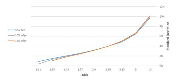We can see clearly that variance increases as the odds lengthen (or as implied probability decreases), in line with the analysis above. From the chart above, making 1,000 1 unit bets with 10% edge has a standard deviation of 6.5% if all bets are made at 5.0 compared to 2.5% betting at 1.67. In both cases the expected return is +100 units (+10%).

An interesting result is that for odds shorter than 2.0, as edge (and thus expected return) increases, standard deviation actually decreases. Finding an increasing edge in odds shorter than 2.0 is rewarded not only by the increase in expected return but with a reduction in variance.

Summaries to be drawn from the data

This article has examined the relationships between odds, edge and variance by simulating a series of bets with a positive edge.

While a larger edge and number of bets increases the likelihood of outrunning a period of bad luck, it is important for sports bettors to understand what type of bettor they are, and to be able to quantify their edge.

This will allow them to more easily avoid being discouraged during a downswing or succumbing to overconfidence biases when results run in their favour.

While a bettor may not know their precise edge at the time of placing each bet, previous Pinnacle articles have discussed reasons for using Pinnacle’s closing price as a measure of the true price.

If the closing price can consistently be beaten, Pinnacle’s low margins mean it is likely that a bettor will generate a positive long-term return.

If a bettor is able to generate a long-term profit betting at Pinnacle’s closing prices however, it may be that they have found an inefficiency that the market fails to incorporate. Pinnacle’s policy of welcoming winners ensures that an edge remains available to any bettor for as long as it exists.

MORE: TOP 100 Online Bookmakers >>>

MORE: TOP 20 Bookmakers that accept U.S. players >>>

MORE: TOP 20 Bookmakers that accept Cryptocurrency >>>

Source: pinnacle.com